Batch Serving Views - Blue Green Databases
This post is part of a Series on the Lambda Architecture. It was written in collaboration with Boxever and first posted on Medium.
Overview
Blue-green deployment is an approach to replacing an active system with a newer version, without impact to production availability. In particular, blue-green database deployment means replacing an active dataset with a new one in an atomic operation without impacting incoming queries. This is critical for the Lambda Architecture which relies heavily on the ability to rebuild views. While rebuilding, we do not want our response times to dive. Similarly, we want the dataset preparation and refreshing to be as fast as possible at a scale of over 1 billion rows. In the case of batch views, the dataset is also read-only which is critical for thinking about solutions and optimisations which may otherwise not work (remember that in the Lambda approach, real-time changes are merged with the batch view later on). The approach we took was inspired in a large way by SploutSQL which is the only true blue green database solution we have come across, and which described the reasons for choosing a blue green database deployment architecture. These requirements include
- Read only
- Atomic switch and rollback
- Key-value
- Fast offline creation of database files
- Zero impact to serving during switch
- Scalable horizontally - partitioned with single partition access per query
- High availability - replicated partitions
- Easy Operations - cluster resizing or maintenance on next switch
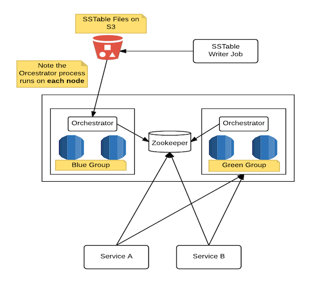
Batch Views - Blue Green Architecture
We achieved the above architecture on datasets with over 1 billion unique keys and 2TB of compressed data, with a p95 latency under 5ms and capable of well over 1k QPS by serving the data on just four m4.xlarge instances with the replication factor set to 2. The instances had SSD based gp2 EBS volumes attached. Our limiting factors for preparation of the blue group nodes was the network card on the m4.xlarge instances (90 MBytes/sec). Downloading from S3 within the EC2 network is exceptionally fast and scalable! So how did we do this?
What Database did we use?
We spent some time researching which databases satisfied the requirements. One option that ticked most of the boxes and had operational tooling built in for blue green deployments was SploutSQL which we already mentioned we took inspiration from. SploutSQL is backed by an SQLite database. Our basic key-value usage with a relatively large but widely varying value column size would be difficult to make work well with a RBDMS. As to be expected, SQLite is more suited to when you need the power of SQL with batch views. As of version 3.x of SQLite, it is one of the few RBDMS systems that store BLOBs inline by default regardless of the size. However, there are performance trade offs in both performance and storage with inline blobs. The only configurable property available in most RBDMS systems for this trade off is the database page size (see here). See the following page for a benchmark regarding inline blob performance with blob size using SQLite. Based on the benchmark it was apparent that too many of the value records in our dataset would perform poorly inline. However, storing them as external blobs would require additional management and a file per record which is infeasible and extremely slow for a large number of records even when using a modern filesystem like ext4. We considered extending SploutSQL ourselves to work with the database backend we finally chose. However, we decided against it as the change would have taken us more time and resources than we had to integrate.
We also investigated options on AWS such as Redis on ElasticCache and DynamoDB, but they were orders of magnitude too expensive for the quantity of data we needed to store, and did not allow us to write the database files offline which was critical for fast rebuilding. Other options like ElephantDB allowed writing the raw key-store files offline but the latest commit was over 3 years ago. In the Hadoop ecosystem one might look at Hive, which at first glance, appears to covers most of the requirements. However, one must either back Hive with HDFS or S3. S3 is excellent but for high frequency random reads, it would not meet our latency requirements at the p95 range. To use HDFS as the backing for Hive we would need a dedicated HDFS cluster to ensure latencies were met which we did not want to do either for reasons we already discussed in a previous post. Hence, we ruled out Hive.
We then looked at Cassandra again. We had good operations experience with Cassandra and knew a lot of the ins and outs that take time to learn. We also knew that many of our latency concerns and pain points with Cassandra could be eliminated altogether due to the fact the dataset was read-only. Compactions would not be required and, in fact, are disabled. Repairs would not be required either and also disabled. Bloom filters ensured we could scale the number of indexes (records) well beyond the memory limits of a machine while experiencing very little performance impact. We also knew that we could use row caching (which as of version 2.2 was usable). We thought that we could write the SSTables offline. Essentially, it appeared to meet all of our requirements.
One option we did not evaluate at the time but, in hindsight, we would have given more consideration is RocksDB. It has gained considerable favour recently with both Apache Flink and Apache Samza choosing it as the storage engine for their checkpointable state management. As it takes ideas from Hive, it is also quite similar to Cassandra and there are many overlapping features as well as some additional features applicable to this use case such as read-only mode and the ability to restore from S3. We still believe that Cassandra was the correct choice given our existing expertise managing, tuning and debugging it.
As with everything, it was not as simple as it appeared and while it works better than we could have ever hoped, it had its challenges.
Generating the SSTables
Being able to generate the SSTables offline in a distributed manner was essential in order to prepare the SSTables for 1 billion profiles in a reasonable duration. We decided to use Spark for the distributed processing as this made most sense in our stack. We could then autoscale the job on EMR to be able to prepare the data within an hour on 50 m3.2xlarge nodes using the spot market! We hit a few issues when writing the SSTables this way. The writer is based on the CQLSSTableWriter in the Cassandra distribution.
The first issue was that the CQLSSTableWriter implementation buffers to memory only. That is, one can only write an SSTable as large as the memory available to your writer process (sort of silly for a database utility). That means you must trade off the number of SSTables (too many and Cassandra will have problems loading them all), with the size of the SSTable you can create without running out of memory on the Spark executors (so you don’t get OOMs or worse YARN killing the executors container as it’s using too much off heap memory - indeed, the writer uses off heap!).
The second issue was related to ensuring that the SSTables file names were unique. As the CQLSSTableWriter works as if it’s a single process it generates SSTable ids using a static AtomicInteger based counter. That means that CQLSSTableWriter instances running on different Spark executors would generate the same SSTable ids and names which would be a problem when we went to load them onto the Cassandra cluster. We solved this by renaming the SSTables based on a guaranteed unique and monotonically increasing id generating sequence based on the Spark TaskContext partitionId.
The third issue we hit was that the SSTable writer, for some bizarre reason, does not create the bloom filters and expects that you will load the SSTable files into the cluster by streaming them into the cluster. As it streams the table in, it will create the bloom filter files and any other missing metadata. Given the entire reason for writing the tables offline was to avoid having to pass the data through the Cassandra process and cluster, the approach seemed nonsensical (and really slow). We solved this by adding additional logic to build the bloom filters for each SSTable index in the job. Therefore as we processed each spark partition, we created all the necessary files required to immediately download and serve the data from a Cassandra node. We needed to set the bloom filter false positive target to 0.001. This was a good trade off between the size of the bloom filters, the hit rate we needed and the number of row keys (indexes) per index file should a bloom filter miss occur.
Record Partitioning
The next challenge we encountered was partitioning the data. We needed to ensure that as we wrote the records, we obeyed the Cassandra partitioning scheme and that we wrote data which belonged to the same node in contiguous partition buckets on Spark (to ensure we could download contiguous ranges to each Cassandra node from S3).
Cassandra can be used with either multiple virtual nodes (vnodes) or a single token per node. We decided not to use vnodes as it overcomplicates our solution. Vnodes are really designed to simplify scaling out and rebalancing your cluster which we would never require as we could just change the cluster setup on the next blue green switch.
To disable vnodes one must configure two properties in cassandra.yml
initial_token: {unique-per-node}</td>
The initial_token is the start token in the token range that the given node will own. The token range is decided by the token partitioner which is by default Murmur3. This has a range of -2^63 to +2^63. To generate the initial_token follow the Cassandra docs here.
Note that the first node in the ring with the lowest initial_token is responsible for the wrapping range (highest initial_token, lowest initial_token]. i.e. the node with the lowest token accepts row keys less than the lowest token and greater than the highest token (see here).
To take an example: We want 4 nodes with replication factor of 2. This means we have 4 token ranges as each node must own one. Each node will contain its token range and the replica set for another token range (i.e. RF=2).
A brief note on syntax for partition ranges. (MINIMUM, X] means exclusive of minimum, inclusive of X. In particular, we don’t want MINIMUM to correspond to any key because the range (MINIMUM, X] doesn’t include MINIMUM but we use such range to select all data whose token is smaller than X. See Murmur3Partitioner getToken method here (ensure you are viewing the correct Cassandra branch - i.e. 2.2)
This gives us the following token ranges.
A:  (2^32     -2^64]
B:  (-2^64    -2^32]
C:  (-2^32        0]
D:  (0         2^32]

node 0 owns token ranges AD
node 1 owns token ranges BA
node 2 owns token ranges CB
node 3 owns token ranges DC
As we generate the sstables in Spark which has its own partitioning mechanism, we need to ensure that it partitions the data as Cassandra is expecting it. The correct records needs to be in the correct SSTables and placed on the correct node. To ensure this we configure our Spark partitioning so that a record which is destined for a given Cassandra token range will end up in a given Spark partition range. Token -> [l,u].
The following example show how this works. Say we want 1024 partitions in spark job. This will result in 1024 partition folders (buckets) on S3. The records are partitioned into SSTables in each of these buckets as follows
Token Range A gets partitions [0,    255]
Token Range B gets partitions [256,  511]
Token Range C gets partitions [512,  767]
Token Range D gets partitions [768, 1023]
which means,
node 0 gets partitions 0:255    768:1023  (AD)
node 1 gets partitions 256:511  0:255     (BA)
node 3 gets partitions 512:767  256:511   (CB)
node 4 gets partitions 768:1023 512:767   (DC)
Keeping all of the partitioning information in sync between the orchestrator responsible for downloading and serving this data on the Cassandra nodes and the writer can become difficult, so the writer produces a metadata file at the end of the job with the relevant partitioning information defined. This way we can change the partitioning scheme from day to day but still enable automatic reuse of previous days without any manual intervention or mismatches.
Row Caching
As the data is read-only and the same row is typically read multiple times during a user’s session, we take advantage of the row caching feature in Cassandra. In versions prior to 2.1 of Cassandra row caching was problematic. It was also on heap which caused additional memory pressure. As of 2.1, it works great and is off heap. The cache is a Least Recently Used (LRU). The Cassandra cache is not write through which means that any updates to a key will cause the cache entry for it to be invalidated. However, our setup functions in read-only mode which means we never encounter this problem. With row caching enabled, we only pay for the disk read (and index scan in the case of bloom filter miss) on the first access during a guest session. To ensure maximum benefit from row caching you must ensure that you use sticky token routing in the datastax driver. We discuss more about that in the Client section.
Schema Definition
CREATE TABLE IF NOT EXISTS boxever_guest_context.guest_context (
  guest_key text,
  context blob,
  PRIMARY KEY(guest_key))
WITH read_repair_chance = 0.0
AND caching = { 'keys' : 'ALL', 'rows_per_partition' : '1' }
AND dclocal_read_repair_chance = 0.0
AND compaction = {'class':'SizeTieredCompactionStrategy', 'enabled':false}
AND speculative_retry = 'NONE';
Querying the Cluster
As you can see in our architecture, the clients which access the data talk directly to the green cluster. In fact they talk directly to the Cassandra node in the green cluster which own the partition key they are looking for (and fall back to the replica if the primary isn’t available). As mentioned in the Row Caching section this means that caching is also optimal.
As this is a Cassandra 2.2 cluster, we use the Datastax driver for querying it. To support the atomic switching of the reads from one cluster to another (i.e. the blue green switch) the driver listens out for notifications from the Orchestrator via Zookeeper watches. Once it receives a notification that it should switch reads to another cluster, it tests the new cluster for availability and on success it switches reads to work against the new green cluster (the orchestration is more involved than this and we discuss it in more detail in the Orchestration section). The Datastax driver doesn’t support switching the clusters you’re querying from and so we created a library which talks with Zookeeper and acts as a facade for executing queries:
public interface CassandraDriver {

    void start() throws Exception;
    void stop();
    DriverState getActiveState();

}
Users of the library should access the getActiveState() on each query. This DriverState provided access to the session and some other utilities. Using a prepared statement with multiple clusters was also tricky as a prepared statement is bound to a specific cluster. Therefore, the driver facade we provided also needs to support keeping track of prepared statements on a per cluster basis and ensure that a new PreparedStatement is created as required for the given query when the cluster switches (essentially, it clears its prepared statements cache on switch).
import static com.google.common.base.Preconditions.checkNotNull;

import com.datastax.driver.core.PreparedStatement;
import com.datastax.driver.core.Session;
import java.util.concurrent.ConcurrentMap;

public class DriverState {
    private final Session session;
    private ConcurrentMap<String, PreparedStatement> preparedStatementCache;

    public DriverState(Session session, ConcurrentMap<String, PreparedStatement> preparedStatementCache) {
        checkNotNull(session);
        checkNotNull(preparedStatementCache);
        this.session = session;
        this.preparedStatementCache = preparedStatementCache;
    }

    public Session getSession() {
        return session;
    }

    /**
     * <p>This prepared statement cache will always ensure that the prepared statements match both the session and more
     * importantly the cluster you are talking to (as new sessions can point to new clusters in blue / green).</p>
     *
     * <p>Never assume the value is present when performing a get() as this is a new cache with new DriverState which
     * happens on new clusters.</p>
     *
     * <p>Use computeIfAbsent(key, lambda) where the lambda creates the prepared statement lazily.</p>
     *
     * @return
     */
    public ConcurrentMap<String, PreparedStatement> getPreparedStatementCache() {
        return preparedStatementCache;
    }
}
To use token aware routing with the driver, you must define your query in a very specific manner. If not it will fall back to round robin routing without notifying you of any issue! You must ensure that you tell the driver what the partition key is for that SSTable. See the requirements section under Token Aware Routing on the Datastax site. The easiest way is to use named variables in your query but just be sure that the named variable is the exact same as the partition column name you’re querying for as if it is not, the driver is not smart enough to figure it out.
Here’s an example of how to query a sample schema using our driver facade.
CREATE TABLE test.sensor_data(
    id int,
    year int,
    ts timestamp,
    data double,
    PRIMARY KEY ((id, year), ts)
);
DriverState driverState = driver.getActiveState();

//ensure you use correct named variables
String cql = "SELECT * FROM test.sensor_data WHERE id = 1 and year = :year";

// get prepared statement from cache or compute if absent
PreparedStatement stm = driverState.getPreparedStatementCache()
	.computeIfAbsent("query", (k) -> driverState.getSession().prepare(cql));

BoundStatement bound = stm.bind(2016);

ResultSet rs = driverState.getSession().execute(bound);
Orchestrator
The orchestration is managed by a custom python application. This is deployed as a sidecar/co-process on each cassandra node within the blue-green cluster. Zookeeper is used by the co-processes for coordination. Each orchestrator is responsible for the following:
- Downloading the data from S3 for token range the node serves
- Synchronizing on nodes ready (distributed barrier using Zookeeper)
- Validating cluster preparation
- Notifying clients to switch cluster
- Clearing down cluster after switch
There are plans to enhance the orchestrator to also support starting and stopping the instances in the blue group when they’re not needed. This enables costs savings by not having the blue instances idling 90% of the time (i.e. while not being actively prepared for switch over). We did not implement this at the time as our eu-west production cluster was not on VPC and so we could not configure it to have nodes always start with the same IPs which was required for this solution.
The orchestrator application itself is not dependent on any particular data store and it can work with any datastore you can write a DataStoreManager for. Combine that with the ability to start and stop instances and you could easily make this work with AWS Services like Redis, RDS, Redshift etc if they are applicable for your use case.
class DataManager:

    @abstractmethod
    def wait_and_download_data(self): pass

    @abstractmethod
    def cleanup_data(self): pass

    @abstractmethod
    def register_data(self): pass

    @abstractmethod
    def get_dataset_summary(self): pass
Finite State Machines
The orchestration process implements the following Finite State Machines (FSM). It would be easier to visualise graphically, however, due to time restrictions, we did not complete the diagrams for this blog post. Hopefully the textual description will be sufficient to understand the transitions.
Blue to Green
if is blue
    ask data manager to download current dataset (waits if necessary to be available)
        on dataset downloaded
            ask data manager to register data

            on registered
                wait for all nodes in cluster to have data registered

                on all nodes registered
                    update new green connect offer (for this cluster)
                    wait for client ack
                        on client ack
                            if ack OK
                                update green live connect
                                exit with success

                            else
                                wait for attempted re-ack (n nodes so n attempts)

        on no data available after max timeout
            exit with failure
Green to Blue
if is green
    listen for blue-green switch
        on switch
            if no longer green
                allow queries X minutes to drain
                truncate, clean and exit

            if still green
                return to listen for blue-green switch

        if no change after max timeout
            exit with failure
Next in the series - Speed Serving Views