Global Black-Box Optimization applied to Hyper-parameter Tuning
In this post, we discuss the problem of global black-box optimisation. We cover the challenges involved in such an optimisation and recent approaches to solving the problem. While it is not intended as an exhaustive literature review, we do cover a variety of methods and why they may, or may not be applicable to a given problem.
Overview
Global black-box optimisation is the problem of minimising an objective function over a configuration space. This objective function may be based in the physical or computational space. The objective function is either entirely unknown or intractable, and so it is a form of black box optimisation.
More formally, where $ f $ is our objective function, there are $ d $ dimensions, and ${\mathcal X} \subseteq R^d$, we are trying to minimize
The term hyper-parameter is typically associated with a configurable model parameter in a machine learning algorithm. This is to distinguish it from standard model parameters which are automatically learned as part of the underlying model training. The tuning of these hyper-parameters can lead to large differences in the performance of a learning algorithm [4]. Even today, in research publications and in practice, it is common to see researcher’s hand tuning ML model parameters based on manual analysis after each optimisation attempt. The cross validation support in more modern ML package pipelines such as scikit-learn have helped in directing users to attempt to automatically run multiple combinations of their experiment with different configurations. However even then, many do not investigate if the underlying cross validation is selecting the configurations to sample based on an intelligent search optimisation, or simply grid or random search. As engineers and scientists, this makes no sense and is ajar to the entire concept of machine learning, which is intended to take the human out of the loop in either tedious or computationally intensive tasks.
The methods involved in hyper-parameter optimisation can be applied to any search space problem where we have many degrees of freedom (free variables), and a loss function to minimize or maximize. As the title of the post suggests, the theory underlying hyper-parameter optimisation approaches has been derived from more general forms of research in the automated configuration of hard computational problems, and more generally falls under the classification of Global Black-Box Optimisation.
Challenges
The manual exploration of the configuration search space by an expert is a time intensive problem. The exploitation of a successful configuration space is even more time consuming and is frequently forgotten. Even with an expert winding their hours away at the problem, they still may not be able to select an optimal solution. When the number of hyper-parameters becomes large and interdependencies amongst them come into play, finding the optimal solution manually becomes less and less likely, even for an expert in the domain. This leads to the need to formalise the search process, so that it can be systematically solved via a global optimisation method [4].
Complex Search Space
Where there are only one or two hyper-parameters, with a handful of discrete domain values per parameter, the problem can be solved via naive approaches such as trialing every combination of configuration options, i.e. grid search. In fact for very low dimensionality spaces, one should probably avoid more advanced methods, as they are unlikely to yield any benefit. However, when the search space involves even a handful of hyper-parameters with large continuous domains, the number of combinations which must be run in order to have sampled the space effectively with a naive approach grows exponentially. This is known as the Curse of Dimensionality.
Let’s take a few examples. The first example has only two hyper-parameters with discrete domains
$ A \in \{0, 5, 10\} $ and $ B \in \{1, 50\} $ gives,
$ \text{Combinations} = C(A) \times C(B) = 3 \times 2 = 6 $
If the hyper-parameters are instead continuous, $ A \in [0:100] $ and $ B \in [0.01:1] $ and we discretise (quantise) the continuous interval into steps of $ 1 $ and $ 0.01 $ respectively, gives,
$ \text{Combinations} = C(A) \times C(B) = 100 \times 99 = 9900 $
Adding another continuous hyper-parameter $ C \in [0:2] $ and discretise with step size of $ 0.01 $ it gives,
$ \text{Combinations} = C(A) \times C(B) \times C(C) = 100 \times 99 \times 200 = 1980000 $
More generally, if one has $ r $ variables, the $ i^{th} $ of which can take on $ n_i $ values, there will be $ \prod\limits_{i=1}^r n_i $ combinations.
In addition to this, hyper-parameters may be non-separable (i.e. are not additively decomposable). In fact it is highly likely that they are non-separable as that would imply they can be optimized separately. Modelling these dependencies is a non trivial problem and the process of optimising such dependencies is not something humans can achieve past two or three parameters.
Costly Objective Function
As we have seen in the previous section, the problem can quickly become intractable even when the objective function is relatively cheap to evaluate (in the order of milliseconds per evaluation). However, a large class of objective functions are much more expensive to compute and can take minutes, to hours, to days to sample from. Some type of objective functions may even be based in the physical space, such as a lab experiment or exploratory well placement. These physical objective functions are expensive in time, effort and money.
Some examples of objective functions include:
- Deep Learning Models
- Synthetic Gene Design
- A/B Testing
- Oil Well Placement
In addition to the cost of the objection function, other factors which can affect the difficulty of the optimisation process include non-smooth, discontinuous or noisy objective functions. There are varying methods available to combat each of these problems to varying degrees, however, when the function itself is black box, it can be problematic to know such issues in advance.
Naive approaches quickly lose all feasibility even with what appears to be a relatively low dimensionality problem at a first glance. Luckily, the last number of years has seen an increase in research in the area of global black-box optimisation. The success machine learning algorithms, in particular deep learning, have led to an increase in research both in academia and industry. However, too much time was, and still is being wasted on the “art” of hyper-parameter tuning. This has led to dedicated research aimed at turning hyper-parameter optimisation into a science [4]. Once there is a formal, methodical approach, the tuning can be automated allowing researchers to concentrate on other areas. We will discuss some of the approaches available, open source implementations of them, and some usage notes based on real world usage. The discussion is from a practical implementation perspective. Those who wish to dig into the hard core theory can read the original papers linked to from this post.
Discussion of Available Methods
As discussed in the abstract, this post is not intended as an exhaustive report on the available methods and so there are some which we do not discuss. The 4 main types of algorithms we will discuss in this blog post are:
- Grid Search
- Random Search
- Evolutionary Algorithms
- Sequential Model-Based Optimization
- Bayesian Optimisation
- Tree Parzen Estimators
We also briefly mention some related algorithms including Sequential Model-based Algorithm Configuration (SMAC) and Particle Swarm Optimisation (PSO).
Grid & Random Search
To quote the conclusion in [4].
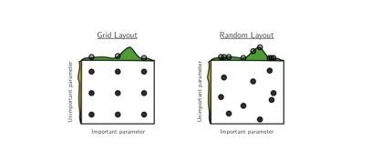
Grid search experiments are common in the literature of empirical machine learning, where they are used to optimize the hyper-parameters of learning algorithms. It is also common to perform multistage, multi-resolution grid experiments that are more or less automated, because a grid experiment with a fine-enough resolution for optimization would be prohibitively expensive. We have shown that random experiments are more efficient than grid experiments for hyper-parameter optimization in the case of several learning algorithms on several data sets. Our analysis of the hyper-parameter response surface (Ψ) suggests that random experiments are more efficient because not all hyperparameters are equally important to tune. Grid search experiments allocate too many trials to the exploration of dimensions that do not matter and suffer from poor coverage in dimensions that are important. Compared with the grid search experiments of Larochelle et al. (2007) [7], random search found better models in most cases and required less computational time. Random experiments are also easier to carry out than grid experiments for practical reasons related to the statistical independence of every trial.
- The experiment can be stopped any time and the trials form a complete experiment.
- If extra computers become available, new trials can be added to an experiment without having to adjust the grid and commit to a much larger experiment.
- Every trial can be carried out asynchronously.
- If the computer carrying out a trial fails for any reason, its trial can be either abandoned or restarted without jeopardizing the experiment.
Grid vs Random Search
Of course there are ways to help both grid and random search with domain knowledge, such as quantising the hyper-parameters to reduce the search space (not the number of dimension). However, these tactics are a crude attempt to work around the underlying optimisation problem.
As discussed, grid search is intractable for all but the simplest of optimization problems. While random search appears to work quite well in practice, it can take a large number of samples to be reasonably confident that a solution close to the optimal has been found. With random search, it is also very difficult to gain confidence that a solution is close to the optimal solution, as there is never a visible convergence in the algorithm. It is however worth noting, that random sampling is still used in some manner, in all of the more sophisticated optimisation algorithms we will discuss in this post.
Evolutionary Algorithms
There are many forms of evolutionary algorithms, from Genetic Algorithms (GA) to Evolutionary Strategies (ES). A GA is an algorithm that is based on natural selection, the process that drives biological evolution. While GAs were very popular in the late 90’s and early 2000’s, they have been superseded by a range of new optimisation algorithms, some of which we discuss in this post. One of the earlier algorithms to succeed GAs was Particle Swarm Optimization (PSO). While PSO and GAs are not the same, they do share some characteristics such as the fact that they are both population-based search algorithms. However, PSO has been shown to perform as well as GA but require fewer evaluations [13].
GAs are characterised by a binary string representation of candidate solutions. Evolutionary Strategies on the other hand use vectors of real valued numbers as the representation. Various types of Evolutionary Strategies exist such as CMA-ES which stands for Covariance Matrix Adaptation Evolution Strategy. Evolution strategies (ES) are stochastic, derivative-free methods for numerical optimization of non-linear or non-convex continuous optimization problems [6]. It is not uncommon to combine with other methods such as Gaussian Processes. It can dynamically adapt its search resolution per hyperparameter, allowing for efficient searches on different scales. When used independently, it is recommended that preferably, no less than 100 times the dimension of the function evaluations be performed to get satisfactory results. If we have tens or hundreds of hyper-parameters, this can be problematic.
Sequential Model-Based Optimization
Sequential Model-Based Global Optimization (SMBO) [4] algorithms use previous observations of the loss function $ (f) $, to determine the next (optimal) point to sample $ f $ for. Both Bayesian optimization and Tree of Parzen Estimator fall into this category.
The advantages of SMBO are that it [8]:
- Leverages smoothness without analytic gradient
- Handles real-valued, discrete, and conditional variables
- Handles parallel evaluations of $ f(x) $
- Copes with hundreds of variables, even with budget of just a few hundred function evaluations
Gaussian Processes are typically chosen as the models for SMBO, but other model types can be chosen such as random forests which are used in the Sequential Model-based Algorithm Configuration (SMAC) algorithm [11]. We discuss only Bayesian Optimization and TPE in this post.
Bayesian Optimization
Bayesian optimization (BO) falls in the SMBO class of algorithms. It has become a very popular field of research in the last number of years, even with a dedicated workshop at NIPS. Some commercial Bayesian Optimisation approaches such as SigOpt indicate that an optimal solution can be found within 20 to 30 times the dimensionality of the optimisation space. This is a very attractive proposition. There are conflicting views on the success of such approaches, but the results are beginning to quell such discussions.
Taking a formal definition from [10]. Let $f: {\mathcal X} \to R$ be a L-Lipschitz continuous function defined on a compact subset ${\mathcal X} \subseteq R^d$. We are interested in solving the global optimization problem of finding
We assume that $f$ is a black-box from which only perturbed evaluations of the type $y_i = f(x_i) + \epsilon_i$, with $\epsilon_i \sim\mathcal{N}(0,\psi^2)$, are available. The goal is to make a series of $x_1,\dots,x_N$ evaluations of $f$ such that the cumulative regret
is minimized. Essentially, $r_N$ is minimized if we start evaluating $f$ at $x_{M}$ as soon as possible.
There are two crucial parts to any Bayesian Optimization procedure approach. Firstly, define a prior probability measure on $f$: this function will capture the our prior beliefs on $f$. The prior will be updated to a ‘posterior’ using the available data. Secondly, define an acquisition function $acqu(x)$. The aquisition function is a criteria to decide where to sample next in order to gain the maximum information about the location of the global maximum of $f$.
Every time a new data point is collected, the model is re-estimated and the acquisition function optimized again until convergence. Given a prior over the function $f$ and an acquisition function, a BO procedure will converge to the optimum of $f$ under some conditions [14].
Gaussian processes are used as the models in Bayesian Optimisation. The best description I have found for what a Gaussian Process (GP) is and why it is useful, is in from the book “Gaussian Processes for Machine Learning” [12].
A Gaussian process is a generalization of the Gaussian probability distribution. Whereas a probability distribution describes random variables which are scalars or vectors (for multivariate distributions), a stochastic process governs the properties of functions. Leaving mathematical sophistication aside, one can loosely think of a function as a very long vector, each entry in the vector specifying the function value f(x) at a particular input x.
It turns out, that although this idea is a little naive, it is surprisingly close what we need. Indeed, the question of how we deal computationally with these infinite dimensional objects has the most pleasant resolution imaginable: if you ask only for the properties of the function at a finite number of points, then inference in the Gaussian process will give you the same answer if you ignore the infinitely many other points, as if you would have taken them all into account! And these answers are consistent with answers to any other finite queries you may have.
One of the main attractions of the Gaussian process framework is precisely that it unites a sophisticated and consistent view with computational tractability.
Gaussian Processes allow us to follow two different types of behaviour - exploitation (sample close to good values we already know) and exploration (sample areas we know relatively little about in case they are better). There are many choices one must make when employing Bayesian Optimisation. These include the covariance function (kernel) of the GP:
- Radial Basis Function, aka Gaussian Function, aka Squared Exponent
- Matérn 3/2
- Matérn 5/2
- Linear
- Exponential
- Brownian
- Periodic
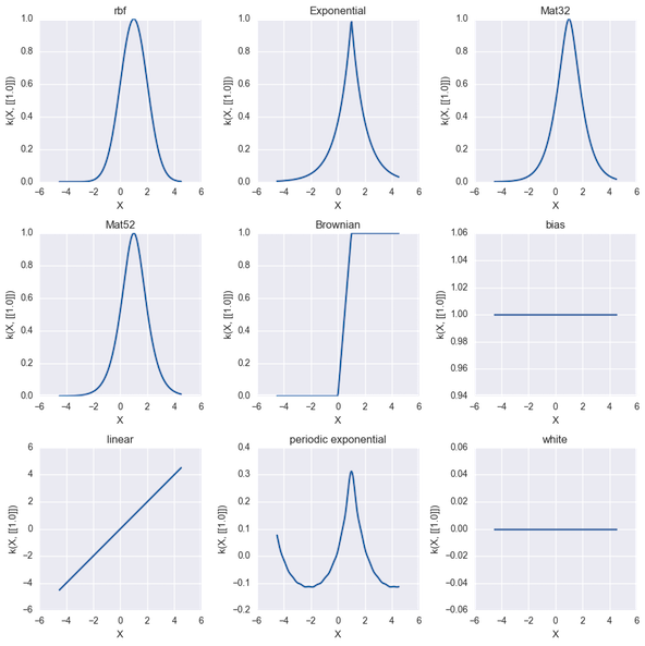
GP Kernels
The Acquisition function which allow us to balance between exploitation and exploration to decide where to sample next:
- Lower Confidence Bound
- Expected Improvement
- Maximum Probability of Improvement
- Thompson Sampling
On top of that there can be varying types of acquisition function optimizers which include:
- L-BGFS
- DIRECT
- CMA
Note that the Limited Memory BGFS (L-BGFS) is designed to work on smooth convex functions. In fact, objective functions are preferably twice differentiable to use L-BGFS effectively, however a locally Lipschitz function is usually sufficient [9]. The Matern 5/2 kernel with Automatic Relevance Determination (ARD) can be used to support a non smooth underlying function being estimated but still be twice differentiable. The standard Radial Basis Function (RBF), aka Gaussian Function has smoothness assumptions that can be excessive for some objectives. It is worth noting that TPE uses CMA-ES for optimizing the acquisition function.
There are many open source implementations available for experimenting with Bayesian Optimisation, including (but not limited to):
We have used GpyOpt extensively. It is an open source Bayesian Optimisation library built on top of Gpy and has a commercially friendly license. Both libraries are produced by the University of Sheffield. We found its support for including constraint information in the domain space definition second to none (see here). It is very well documented (see here and here), and has many options for the model and acquisition functions. They also have a Spearmint interface which allows running existing Spearmint processes by changing only a single line of code. We have not used Spearmint or BayesOpt due to their non commercial friendly license.
The theory behind Bayesian optimisation has been around for a long time. However, it had some practical problems. In particular, the number of hyper-parameters for the Bayesian optimisation process itself. These are different from the hyper-parameters of the underlying optimization problem. They include the model type, kernel type (covariance function), the acquisition function, the acquisition function optimizer and associated variables such as exploration jitter. The most important of these are the covariance function parameters such as the length, variance and noise. Fortunately, a fully bayesian treatment of the problem has been developed that marginalises over the covariance function hyper-parameters and computes the integrated acquisition function. This leads to an integrated acquisition function corresponding to a Monte Carlo integration over the individual acquisition functions of each GP, for which we use the expected improvement. The estimate of the optimal point at any step of the algorithm is given by the point of those queried with the maximum mean value in the GP posterior (with the hyperparameters marginalized out).
As choosing such an approach to integrating out the GP hyperparameters means choosing Expected Improvement as the acquisition function, it reduces the number of choices one must make and the improves the automation of the optimization solution further. However, there are still variables such as kernel type and acquisition jitter which must be tuned and can have a large effect.
While some Bayesian Optimisation libraries hide the complexities involved in the process almost completely, we have found that it is beneficial to spend some time studying the theory behind Bayesian Optimisation before trying to use it for hyper-parameter optimization. Using somewhat lower level libraries such as GPyOpt require one to be familiar with the theory discussed above in order to utilise the library efficiently. There are a number of commercial offerings arising and various high profile purchases of startups by the likes of Twitter in recent years. This demonstrates that using Bayesian Optimisation effectively is not a trivial matter. SigOpt itself was based on MOE which was developed at Yelp to optimise A/B testing. To provide you with an insight into the roots of SigOpt and why they started the company we have taken a snippet from here
We are similar to hyperopt, spearmint, and MOE, which we developed at Yelp and also uses Gaussian Processes to do Bayesian Global Optimization. SigOpt extends and expands upon our work on MOE while wrapping everything in a simple API and web interface. One thing we learned while promoting MOE was that many people have this problem, but few have the time or expertise to get these expert level open source tools running properly, so we built SigOpt to bring these powerful tools to anyone via a simple API.
Tree of Parzen Estimator
Another form of SMBO algorithm is the Tree of Parzen Estimator (TPE). Whereas the Gaussian process based approach modeled $ p(y|x) $ directly, this strategy models $ p(x|y) $ and $ p(y) $ [4]. $ P(x|y)P(x|y) $ is modeled by transforming the generative process of hyperparameters, replacing the distributions of the configuration prior with non-parametric densities. The TPE algorithm scales linearly in the number of dimensions being optimised. Interestingly it uses CMA-ES to optimise the continuous hyper-parameters [4].
HyperOpt is a python implementation of the TPE algorithm by the author of TPE. It has support for defining conditional configuration spaces, various parameter distribution types and even has support for distributed sampling. The distributed sampling code feels a little stale and could be easier to use (e.g. the optimisation function code could be transmitted to the workers automatically, instead of having to manually distributed and append the code to the path on the worker processes). However, all things considered it is a very nice library to use and easy to get up and running on custom problem domains within a couple of hours.
We have found the TPE algorithm to be a simple and very effective optimisation method to obtain competitive results on a variety of problems. It requires slightly more evaluations than Bayesian Optimisation but is much easier to start working with.
Final Notes
There are a number optimization libraries which allow one to test a variety of these optimisation algorithms, and some others which we don’t specifically mention here such as Particle Swarm Optimisation (PSO). Optunity is an example of such a library. While we have not used this library, it appears to provide an elegant and common interface over a variety of hyper-parameter optimisation approaches (what it calls solvers). An excellent comparison and overview between the different approaches and various implementations can be found here. It compares the approaches both with varying numbers of dimensions and smoothness.
Hyper-parameter optimization does not free you from the traps associated with machine learning algorithms such as overfitting. As with all machine learning and optimisation problems, one should ensure that the model is not overfit. One can and should include the out of sample evaluation as the output of the objective function to ensure that this is taken into account by the optimisation process.
Visualising Optimisation
As with every problem, it is useful to visualise the progress and results in an intuitive manner. Some hyper-parameter optimisation methods lend themselves well to visualising optimisation results while others do not. Random search for example will not allow one to visualise any discernible pattern in the progress of the optimisation. However, SMBO algorithms such BO and TPE have properties that mean a convergence towards a global optimum should be visualisable. In fact, if a convergence is not visible with these methods, it may signify that it has not found a suitable configuration to exploit, and may either require more evaluations, or another tweak.
Two plots we have found particularly useful for visualising the performance / convergence are scatter plots with the associated kernel density estimate distribution plot for the given hyper-parameter. Again, depending on the optimisation algorithm employed, there may be varying patterns in this convergence. Similarly, there may be random samples and what appear to be resets where a convergence is found but the algorithm then attempts to sample outside of this space (i.e. exploration).
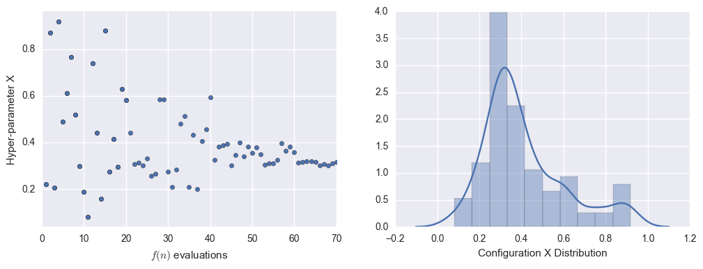
Configuration Convergence
[1] F. Hutter. Automated Configuration of Algorithms for Solving Hard Computational Problems. PhD thesis, University of British Columbia, 2009.
[2] F. Hutter, H. Hoos, and K. Leyton-Brown. Sequential model-based optimization for general algorithm configuration. LION-5, 2011.
[3] Bergstra, James, and Yoshua Bengio. Random search for hyper-parameter optimization. The Journal of Machine Learning Research 13.1, 2012.
[4] Bergstra, James S., et al. Algorithms for hyper-parameter optimization. Advances in Neural Information Processing Systems, 2011.
[5] Močkus J. On bayesian methods for seeking the extremum. Optimization Techniques IFIP Technical Conference Novosibirsk, 1974.
[6] N. Hansen. The CMA evolution strategy: a comparing review. In J.A. Lozano, P. Larranaga, I. Inza, and E. Bengoetxea, editors, Towards a new evolutionary computation. Advances on estimation of distribution algorithms, pages 75–102. Springer, 202006.
[7] Larochelle, D. Erhan, A. Courville, J. Bergstra, and Y. Bengio. An empirical evaluation of deep architectures on problems with many factors of variation. ICML’07, pages 473–480. ACM, 2007.
[8] James Bergstra et al. Computational Science & Discovery Vol 8, 2015.
[9] Lewis, A.S., Overton, M.L. Nonsmooth optimization via BFGS, 2008.
[10] https://github.com/SheffieldML/GPyOpt/blob/master/manual/GPyOpt_reference_manual.ipynb
[11] http://www.cs.ubc.ca/labs/beta/Projects/SMAC/
[12] Carl Edward Rasmussen and Christopher K. I. Williams. Gaussian Processes for Machine Learning. The MIT Press, 2006.
[13] Rania Hassan, Babak Cohanim, Olivier de Weck. A Comparison of Particle Swarm Optimization and the Genetic Algorithm, 2005.
[14] Adam D. Bull. Convergence rates of efficient global optimization algorithms. JMLR, 2011.